Tips for Excel, Word, PowerPoint and Other Applications

VLOOKUP-MATCH Combos

Why It Matters To You

We've previously discussed VLOOKUP as a way to match items against a list and return a corresponding value by specifying which column in the LOOKUP array we want data retrieved from. VLOOKUP does this pretty well, but a lot of times we hard code the column reference, making the function somewhat static. What if we want to select a value from a table? What if, instead of simply picking a sales region, we also want to select the quarter or product line? In some cases, we might not even know what column we need to pull from.

How To ...

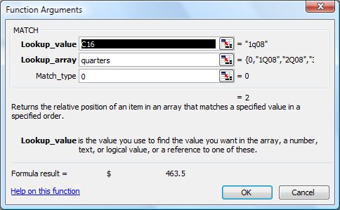
The MATCH function returns the relative position of a lookup value from the specified value in a lookup array. This means that if my lookup value is X, MATCH will look across the specified cells, including blanks, until it finds X and then tell me the relative position where it was found. The relative position is returned as 1 - n, where n is the total number of cells in the array row or column.

This might be a little easier if you download the example sheet, vlookup_match.xls.

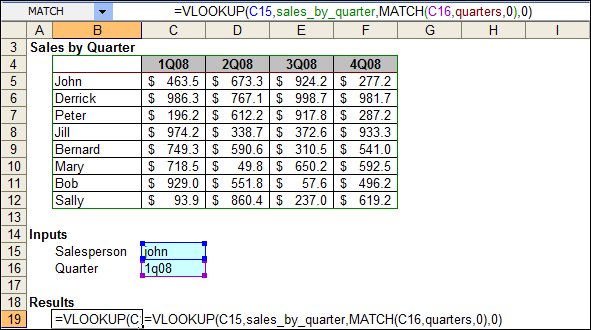
So how does the combo really work? Let's say I have 8 salespeople and I want to return their sales for a particular quarter. I can either use a VLOOKUP to look up by Name or I can use a HLOOKUP to lookup by Quarter, but how do I find the intersection of the two? Let's stick with VLOOKUP for this example, but using the HLOOKUP option is just as easy. If I use VLOOKUP, then I need to dynamically change my column reference to return the right value corresponding to the quarter.

This is where MATCH comes in. I can replace the VLOOKUP's column reference with a MATCH function tied to an input box (C16), where I specify which quarter I want to report on. The named range, "quarters", refers to cells B4:F4. I specify 0 as the match type, because I'm only interested in exact matches. So, when Excel tries to find the value 1q08 in my header row, it finds it in the second cell of the range and therefore returns a value of 2, which then tells my VLOOKUP function to use the value in column 2.

You might be wondering, why did I include the blank cell, B4, in my MATCH array. Remember, the first column of a VLOOKUP array is always the lookup column. If I had not used the blank cell, I would have had to add one to the MATCH value in order to make the VLOOKUP reference the correct column.

You can take this one step further by using data validation to control your inputs and make sure your users don't break anything. There is an example of this in the example file linked above.

Notes

Last updated	8/15/08
Application Version	Excel 2003
Author	Michael Kan
Pre-requisites	None
Related Tips	Introduction to VLOOKUP Data Validation in Excel