
Tips for Excel, Word, PowerPoint and Other Applications
INDEX-MATCH Combos
Why It Matters To You
We previously discussed one method of looking up a value from a table using a VLOOKUP-MATCH combo. This works when have a specific value for which you want an associated value. The INDEX-MATCH combo is another way to look up a value from a table, but this works when you don't necessarily have a LOOKUP value. Trust me, it's easier just to get into it.
How To ...
In this example, I'm going to use a table of bids as my example data set.
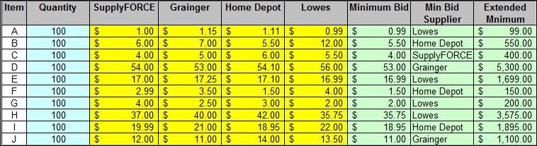
You can also take a look at the example file, index_match.xls. We're going to use our combo to automatically identify the lowest cost bidder for each line item because the first thing every manager wants to know after RFP's are recieved, is the potential savings for each? You can automatically generate this information by combining two simple functions: INDEX and MATCH.
INDEX returns a value given a table or range of values, row #, and column # you have specified. For example, in a 3 x 3 array, I can tell Excel to pick the value from the second column, second row. Simple enough?
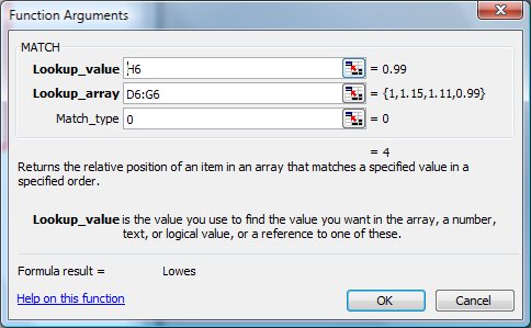
MATCH was discussed in a previous tip, VLOOKUP-MATCH combos, but here it is again. MATCH returns the relative position of an item in an array that matches a specificed value in a specified order. We're going to use the MATCH function to determine which supplier made the lowest bid for each line item.
How are the formulas used in this example?
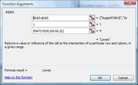
Here is the formula used the determine the low bid supplier for item A:
=INDEX($D$5:$G$5,1,(MATCH(H6,D6:G6,0)))
- For each line item (A-J) we will first determine the minimum bid using a simple MIN function.
- Next, we will MATCH the minimum bid to the range of bids for each line item and determine the relative position of the minimum bid. This will return a numerical value that corresponds to its order in the set of bids received. For example, if the SupplyFORCE made the minimum bid, then the returned value would be 1, since it is the first bid in range. However, if Grainger made the minimum bid, the returned value will be 2.
- The INDEX function is used to return a supplier name, we just need to know which one to return.
- So, we will use the returned value from our MATCH function to specify the column variable in our INDEX function.
- If you feel lucky or are limited by the number of columns you can use, you can also replace the lookup value with a nested MIN function.
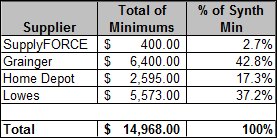
Lastly, we'll finish this exercise by using a simple SUMIF to quickly summarize the total value of each supplier's bid
Notes
| Last updated | 8/15/08 |
| Application Version | Excel 2003 |
| Author | Michael Kan |
| Pre-requisites | None |
| Related Tips |
Basic COUNTIF/SUMIF Named Ranges VLOOKUP-MATCH Combos |