Tips for Excel, Word, PowerPoint and Other Applications

Conditional Formatting: Formula Is

Why It Matters to You

In the precursor tutorial, Conditional Formatting: Cell Value Is, we talked about how Conditional Formatting based on the cell's value is a powerful tool for drawing attention to specific pieces of data. If you bought that argument, then I think you'll agree that Conditional Formatting based on the results of a formula is even more powerful? Why? Often times, the reason we want to highlight a cell doesn't reside in the cell itself or is more complex than a single cell.

How To

Start by opening the sample file called conditional_formatting_formula.xls. In this file, I've created 3 examples that I use on a regular basis that should help you understand how this works.

To launch the Conditional Formatting Wizard, go to the Main Menu, select Format: Conditional Formatting (ALT, O, D). Now select Formula Is from the dropdown. Once you do this, you'll be presented with a place to write your formula.

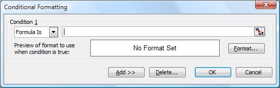
The formula has to be in the format of a test that can be answered TRUE or FALSE. If the result is TRUE, the formatting will be applied. If not, then Excel will move on or keep the default formatting. This may be a little confusing at first, but think of it this way; I can't simply write a VLOOKUP formula, like LOOKUP a value, I have to write a VLOOKUP formula that compares the returned result against a criteria. For example, use VLOOKUP to return a value and test if it is greater than x. This is a question that can be answered as TRUE or FALSE. Let's take a look at a couple of examples.

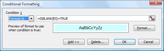
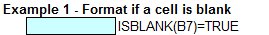
A common use of Conditional Formatting I often use is to turn a cell blue if it is blank. I do this to highlight cells that must be filled in by my survey or RFP respondants. As soon as they provide an input, the shading goes away, which makes it very easy to identify cells that still need a response. The formula is written with a ISBLANK function. If the cell is blank (ISBLANK), it will return TRUE, and FALSE otherwise. If the formula returns TRUE, the conditions are met and the cell is shaded blue. If the formula returns FALSE, the conditions are not met and no formatting is applied, i.e, the blue shading is turned off.

This is what the result looks like. You can go into the sample file and try it out. One thing to notes is that when I specified B5 as the target cell, I used a relative reference. This allows me to use the format painter to apply this conditional formatting to any other cell I want and each cell will test on its own state.

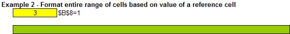
The next example allows you to highlight a range of cells based on the results of a single cell. Sometimes you want to highlight an entire row or column based on the result of a target cell. This looks very much like the 3-part conditional formatting we saw in the basic tutorial, but the formula allows all cells formatted with this schema to test against the same cell. Notice in this example, that I'm using an absolute reference because I want all of my formatted cells to format based on the results of B8. If I were formatting a number of rows, I might change this to a mixed reference where the either the column or the row as absolute and the other remained relative.

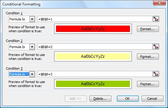
Here's the final result. Based on the value in the yellow-shaded cell, the entire green bar will turn red, yellow, or remain green. You can also use data validation in the yellow-shaded cell to ensure the user is restricted to numbers that will trigger the conditional formatting.

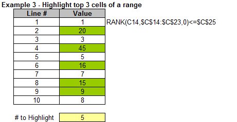
The last example is very cool. The formula tests the rank of each cell against a specified range and only highlights the top X values, where number of cells to be highlighted is controlled by the yellow-shaded cell.

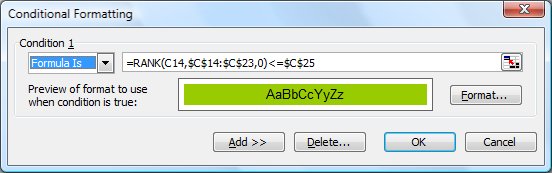
Here's the example. Open the sample file and try changing the values in the example or change the # to Highlight value and see how the shading changes.

Hope this all makes sense.

Notes

Last updated	3/16/08
Application Version	Excel 2003
Author	Michael Kan
Pre-requisites	Conditional Formatting: Cell Value Is
Related Tips	RANK, LARGE, and SMALL - more useful functions you've never heard of Scorecards in Excel ISBLANK