
Tips for Excel, Word, PowerPoint and Other Applications
Conditional Formatting: Cell Value Is
Why It Matters to You
Conditional formatting allows you to change the font, border, or shading of a cell based on up to 3 conditions. When combined with the default color, this allows a cell's format to assume up to 4 states based on the contents of the cell. This becomes very useful when you or your user needs to quickly identify specific pieces of data. Combine this with a relative reference for the conditional test and now you have a mechanism that allows your user to quickly identify any cell that meets their specification.
How To
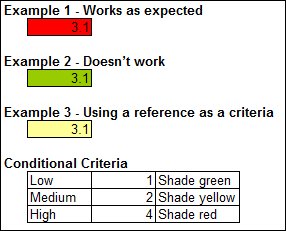
Start by opening the sample file called conditional_formatting_basic.xls. The exercise file contains 3 simple examples using the Cell Value Is function. The first example is a simple 3-part conditional format using hard figures, the second one doesn't work, and the last one is built using references.
To launch the Conditional Formatting Wizard, go to the Main Menu, select Format: Conditional Formatting (ALT, O, D). You can specify formatting based on the cell value or the results of a formula. This tutorial will only focus on conditional formatting based on the cell value.
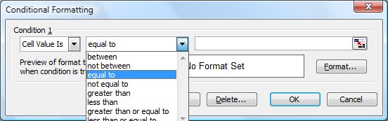
Ensure the first drop down is set to Cell Value Is. The next drop down allows you to specify the relationship of the cell value to the specified value. You can make the formatting conditional on the cell value being equal to, not equal to, less than, etc the test value. In this example, we want to apply the formatting if the cell's value is greater than the test value.
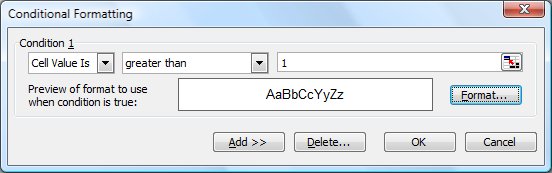
The next step is specifying your test value. In this case, we're going to a value of 1. Therefore, the formatting we select will only be applied if the cell's value is greater than 1. Simple enough?
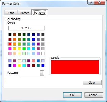
Click on the Format button and the Format Cells window will open. This allows you to select formatting to apply to the cell if the contents meet the test conditions. We're going to turn the cell red when the cell's contents are greater than 1.
To add another conditional test, simply click the Add button or the Delete button to get rid of a condition. Now, order of tests is important. Excel will test the cell's contents against the first condition, determines if it meets it or not and if it doesn't moves onto the next condition. If the cell's contents fails all tests, it retains the default formating.
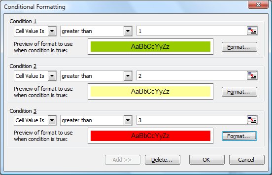
Here's an example of a 3 condition format that tests the cell's contents to see if it's greater than 3, 2, or 1 and turns the cell's color red, yellow, or green accordingly.
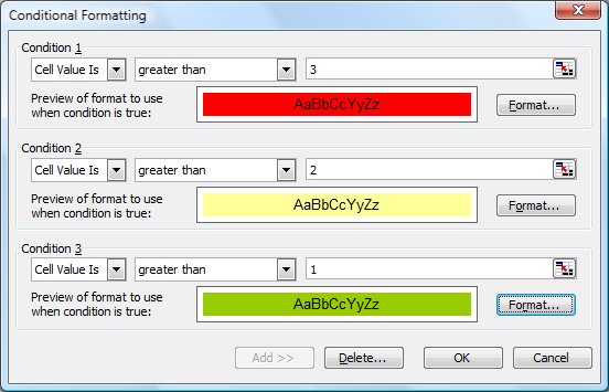
If I reverse the order of the conditions, my formatting won't work. Why? If the cell has a value of 3, it tests against the first condition (e.g., greater than 1), which it meets, and therefore receives the green formatting. So, any cell that is greater than 1 will be turned green and no cell will ever be turned yellow or red.
A Little More Advanced
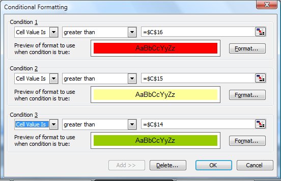
You can get much more sophisticated by simply using variables instead of hardcoding the numbers in the Conditional Format wizard. Here is the same 3 conditional tests, but instead of using values of 3, 2, and 1, I've referenced a set of cells that contain the values 3, 2, and 1. "But that's the same thing" you say. Yes, but not exactly. I'll concede that it's the same thing for now, but if my user wants to raise the threshold for turning a cell red to 5, they can do it by changing a single cell, thus allowing some very nice flexibility and user friendliness to the worksheet.
Here's what the excercise worksheet for this last example looks like. I have the same conditional formatting specified with a simple table showing the conditional thresholds below it ... or you could move this to a control panel page somehwere.
Hope this all makes sense.
Notes
| Last updated | 3/1/08 |
| Application Version | Excel 2003 |
| Author | Michael Kan |
| Pre-requisites | None |
| Related Tips |
Conditional Formatting: Formula Is |