
Tips for Excel, Word, PowerPoint and Other Applications
RANK, LARGE, and SMALL - more useful functions you've never heard of
Why It Matters to You
Need to rank spend by business segment, by supplier, by GL code? Does your boss keep asking, what are the top 10 expense lines? Need I say more? RANK, SMALL, and LARGE are three functions that can help you with this analysis. These are also useful if you do a lot of home budgeting, review of credit card statements, etc, to rank top expenditures.
How To
Open the example file, ranking_functions.xls as a reference. For purposes of this article, I'm going to use a supplier bid example to discuss the ranking of values, but these functions work equally well whenever you need to rank order criteria, such as sales, expenses, ratings, etc.
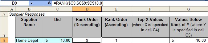
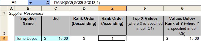
RANK returns the relative rank of a given value from an array of numbers. Rank can be specified in ascending or descending order.
For example, the formula =RANK($C9,$C$9:$C$18,0) will look at cell C9 and tell you how it is ranked, in ascending order, out of all the values in the range C9:C18.
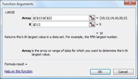
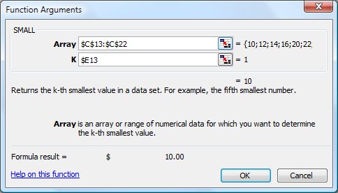
LARGE and SMALL look at array and return the Nth largest or smallest value in an array, where N is a number you specify.
For example, the formula =LARGE(C9:C18,2) will return the second largest value in the range C9:C18 while the formula =SMALL(C9:C18,2) will return the second smallest value in the range C9:C18.
These three functions can be used to rank order or identify supplier response and help you quickly identify a number of low bidders. For example, if I want to identify the lowest three highest bidders or the 5 lowest bidders, I could use a table and sort criteria, but this isn't very dynamic and I might not want to change the layout of my data.
Here's an alternative, using RANK, LARGE, and SMALL. First, I use variables (yellow-shaded cells) to set the number of low or high bids I want to see. I use variables because you may want to change your sorting criteria dynamically. Play around, change the numbers, and see what happens in the Supplier Responses Table.

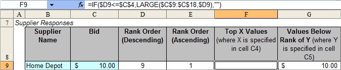
Next, I use the RANK, SMALL, and LARGE functions in addition to a simple IF statement to pull out the top x or lowest y values. The data in the blue cells is the raw bid data.
Here is a simple RANK formula, which evaluates rank in descending order ...
... and the same, which evaluates rank in ascending order. Note that only the last argument is different.
Here is a LARGE function paired with an IF. The object of this formula is to only present the value if it is in the top x values, otherwise return a blank.
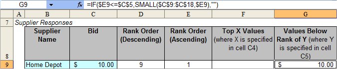
The converse of the above formula presents the value only if it falls within the lowest x of values, otherwise return a blank.
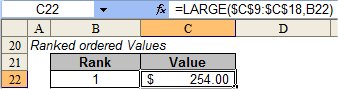
This last example just allows me to rank order the bids in descending order, without having to sort my underlying data set, which could be large and ugly. NOTE. You will run into problems if you have two entries with identical values.
Notes
| Last updated | 8/24/08 |
| Application Version | Excel 2003 |
| Author | Michael Kan |
| Pre-requisites | None |
| Related Tips | Highlighting the Top N Values |